Cheapest place

Solve the small system with cheapest-place algorithm.

For this tutorial we need following modules:

from prp.solvers.simple import CheapestPlaceSolver, CostsType
import prp.recorder as recorder
import prp.xy as xy
import prp.utils as utils

Parameters

We define paths to JSON files of the small warehouse system

LAYOUT_FILE = "../data/10-layout.json"
INITIAL_STATE_FILE = "../data/10-initial-state.json"
DEPARTURES_FILE = "../data/10-departures.json"

and store the solution to a JSON file:

SOLUTION_FILE = "../data/solutions/10-cheapest-place-solution.json"

Calculate

Load the warehouse model from JSON files.

def load_problem():
    """Load a test system with 10 places and 10 pods randomly distributed among them."""
    layout = xy.Layout()
    with open(LAYOUT_FILE, 'r') as infile:
        layout.load_from_json(infile)
        warehouse = layout.get_empty_warehouse()
        costs = layout.get_costs()
        warehouse.set_costs(costs)
    with open(INITIAL_STATE_FILE, 'r') as infile:
        recorder.load_initial_state_from_json(infile, warehouse)
    with open(DEPARTURES_FILE, 'r') as infile:
        departures = recorder.load_departures_from_json(infile)
        warehouse.set_departure_generator(departures)
    return warehouse


warehouse = load_problem()

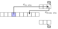
Components of the costs.

When a cheapest-algorithm chooses a place it selects a place with the lowest costs. It makes only short term decision and ignores consequences for the future decisions. Before we can use this algorithm we need to decide what kind of costs we want to compare:

• For costs in only one direction – to storage – use CostsType.FROM_STATION_ONLY. On the costs figure they are marked as \(c_{\text{from stn}}\). The NearestPod algorithm in RAWSim-O uses this type of costs. They are easy to calculate and they work when we cannot predict the future departure of the pod.
• For costs in both directions – to storage and from storage – use CostsType.DECISION. These costs represents the costs full costs for a single decision. On the costs figure these costs correspond to the sum \(c_{\text{from stn}}+c_{\text{to stn}}\). You can use these costs only you know the future departure of the pod.

In the small test system, the cheapest place will return the same results for both types of the costs. In fact, the small test system were deliberately constructed to have this property. But, in general, the cheapest-place returns different results for different type of costs.

In this tutorial we will consider only the costs from and to the station.

solver = CheapestPlaceSolver(warehouse, costs_type=CostsType.DECISION)

We run the system with our cheapest-place solver and record solution.

solution = []

while not warehouse.finished():
    place_id = solver.decide_new_place()
    solution.append(place_id)
    warehouse.next(place_id)

Finally we print the results and store the solution to a JSON file.

print("Total costs: {} at time {}.".format(warehouse.total_costs, warehouse.t))

# Save solution to a JSON file.
utils.create_missing_directories_of_file(SOLUTION_FILE)
with open(SOLUTION_FILE, 'w') as outfile:
    recorder.store_solution_to_json(solution, outfile)